Practical teleportation is not without its complexities.

Bouncing effortlessly around the world requires connectivity data on global networks. manaOS utilizes a datapack (the shaping.db file) with a picture of global networks based on Netflix devices - unfortunately this is very difficult to produce. Most of these complexities are discussed in great detail in previous talks - the difficulty revolves around needing packet loss, latency, bandwidth, and how those change over time during the course of a day and week. Many broadband and cellular networks exhibit high and low congestion periods, networks change over time as links are added or removed, and large scale population events (such as the Olympics or FIFA matches) occasionaly cause singularities in the data.

After handling this, some of the primary variables that we need, such as packet loss, is not directly measurable. Normally we infer this hidden parameter based on either timeouts or retransmits, but no packet that we have ever seen shows up in a counter saying, “by the way, I was lost!” Even a simpler parameter like bandwidth is computed based on transferred bits over time, with handshaking and TCP window scaling contributing outsized influence on the bandwidth of small (vs. large) transfers.

The mix of different internet pay packages and devices (with wildly different network stacks and computation speed for TLS challenges) add on additional modeling difficulties when trying to separate direct network effects from bandwidth capping or other payment artifacts. Even after correcting for all of that, the earlier version of the Netflix app didn’t have the kernel level instrumentation available to directly observe packet retransmit rates (RTX) on most platforms.

Choosing a metric to determine the quality of the datapack was a topic for debate, and ultimately determined not to be a blocker to the initial release as it was assumed we would be iterating rapidly on improving the data vs. a growing set of ground truths. The ground truths represent either direct network measurements from data sources outside of the Netflix application using more traditional network tools such as iperf3, traceroute, tcp/icmp ping, and similar. The initial set of ground truths was highly biased by quality office connectivity, and that led to modeling difficulties when comparing the modeled ISP parameters against real measurements in the field. We refer to this the first public model, as it was released on the manaOS repo.

Practice, of course, rarely follows expectation.

By the time this datapack received public review outside of the office, most of the earlier staff were already working on other projects, serving as another stepping stone on the warning path of “Release Early, Release Often”.

In its present state, the datapack is unusable by the project. Manual values can still be inserted into the database based on known-good ground truths, but the majority of the data appears to be off by a scale factor of a few orders of magnitude, in need of modeling improvements. As a short term fix, if we know the modeling inaccuracy in the current datapack, building a lower quality simulation is possible by applying a piecewise rescaling function as can be seen here:

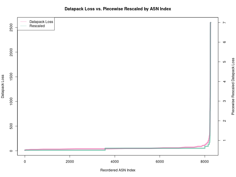
(Note that corrected is clipped to 0.1 tolerance)

This graph shows every ISP (actually the ASN) in the datapack sorted by raw packet loss with low loss ISPs are on the left and high loss on the right. Using lightly verified ground truth data (insufficient quality to model with), a few ISPs from the right appear to be proportionally different to a few ISPs on the left, but without proper rigor, we can’t (in good confidence) rebuild the datapack from such a small sample of unverified data.

To move ahead on the manaOS development, the production of the datapack was decoupled from the release of the operating system. Plugging ground truths from high confidence network measurements into the system allows the end-user the ability to accurately simulate and quickly teleport between the known-good datapoints.

So what is the corrected line?

The raw (unsorted) data looks more like this, comparing AWS and OpenConnect loss (OpenConnect servers provide direct measurements on the server side of retransmit rates / RTX for useful comparison):

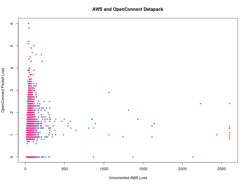
This chart (based on the released shaping.db) gives an idea of the variability in the modeled ISP measurements, which vary over several orders of magnitude, and ignoring the units of the data, seem to indicate where local CDN peering varies greatly from the path to the business logic servers, which has support from some unpublished secondary metrics (such as DASH streaming flows, license and log data transmit times, and similar).

The color shows a simple k-means clustering (4 clusters) of this data, used to derive a piecewise rescaling factor, which is then applied to move the earlier raw packet loss line (left y-axis) to the corrected line (right y-axis). This correction model is overly simplistic (“correction” itself is probably too strong a word), but it serves as a starting point to put the raw data into approximately the right codomain.

It’s very important to note - this is not a proper fix, and that’s the reason we will be leaving the warning notice on the front page and parts of the website about the data quality. The hope is that this provides a more useful starting point for development, and the manaOS community will have time to engage in more detail with the challenge.

Early work on Corrections

While an interface hasn’t been added to do this yet, applying the changes to shaping.db is relatively easy at the command line. manaOS copies its existing shaping.db over to the ephemeral /tmp during boot where updates can be applied without modifying persistent storage:

# to modify the shaping data for an ASN in ephemeral storage:
#   for hardware, attach a serial cable and use picocom to enable ssh
#   for virtualbox, the console is directly accessible
# to get the internal IP address:
ip addr br0     # usually 192.168.21.1
# public ip:
ip addr enp1s0


# Check ssh access from your host (not the console):
ssh -p22 root@IPADDRESS

# Backup shaping.db in case of accident (and you don't want to reboot):
cp /tmp/shaping.db /tmp/shaping.db.backup1
cp /tmp/shaping.db /tmp/shaping.db.backup2

# Note that this will be overwritten on reboot:
sqlite3 /tmp/shaping.db
# enable column headers:
sqlite> .headers on
sqlite> .schema shape
CREATE TABLE shape (
  asn INT,
  utchour INT,
  awsdelay INT,
  awsloss REAL,
  akamdelay INT,
  akamloss REAL,
  ocdelay INT,
  ocloss REAL,
  bandwidth INT
);

# ASN 64512 is "Aim High" in the private allocation space
# Let's look at the shape at midnight UTC:
sqlite> SELECT * FROM shape WHERE asn=64512 AND utchour=0;
asn|utchour|awsdelay|awsloss|akamdelay|akamloss|ocdelay|ocloss|bandwidth
64512|0|25.6|23.7|38.7|2.0|0|1.3|22986

# modify aws packet loss to be 1/100th the present value and review:
UPDATE shape SET awsloss=ROUND(awsloss/100.0, 1) WHERE asn=64512 AND utchour=0;
sqlite> SELECT * FROM shape WHERE asn=64512 AND utchour=0;
asn|utchour|awsdelay|awsloss|akamdelay|akamloss|ocdelay|ocloss|bandwidth
64512|0|25.6|0.2|38.7|2.0|0|1.3|22986

Applying the piecewise correction as described above is accomplished with a little more SQL:

# copy over the backup db:
cp /tmp/shaping.db.backup2 /tmp/shaping.db

# Note that this will be overwritten on reboot:
sqlite3 /tmp/shaping.db
sqlite> CREATE TABLE shapecat (asn INT NOT NULL,cluster INT NOT NULL);

# for rescaling, assign
#   "Aim High" (ASN 64512) to cluster 2
#   "Aim Medium" (ASN 64513) to cluster 1
#   "Aim Low" (ASN 64514) to cluster 3
# assign the rest based on your ground truth / correction analysis:
sqlite> INSERT INTO shapecat VALUES (64512, 2);
sqlite> INSERT INTO shapecat VALUES (64513, 1);
sqlite> INSERT INTO shapecat VALUES (64514, 3);

# This query is long, omitting the "sqlite> " prompts
# Applying this piecewise correction from the earlier k-means analysis:
#   Rescale cluster 2 awsloss from 0.5% to 1.2%
#   Rescale cluster 1 awsloss from 1.3% to 3.6%
#   Rescale cluster 3 awsloss from 3.7% to 7.0%
# To simplify, create a `shape2` table for review first:
CREATE TABLE shape2 AS
SELECT
  s.asn, s.utchour,
  s.awsdelay,
  CASE sc.cluster
    WHEN 2 THEN ROUND(s.awsloss / 544.7 * (1.2-0.5) + 0.5, 1)
    WHEN 1 THEN ROUND(s.awsloss / 1640.5 * (3.6-1.3) + 1.3, 1)
    WHEN 3 THEN ROUND(s.awsloss / 2600.0 * (7.0-5.0) + 5.0, 1)
  END AS awsloss,
  s.akamdelay,
  CASE sc.cluster
    WHEN 2 THEN ROUND(s.akamloss / 544.7 * 1.2, 1)
    WHEN 1 THEN ROUND(s.akamloss / 1640.5 * (3.6-1.3) + 1.3, 1)
    WHEN 3 THEN ROUND(s.akamloss / 2600.0 * (7.0-5.0) + 5.0, 1)
  END AS akamloss,
  s.ocdelay,
  s.ocloss,
  s.bandwidth
FROM shape s
  JOIN shapecat sc ON s.asn=sc.asn;

# Review the new table
-- SELECT * FROM shape2;

# If approved, replace the old table:
DROP TABLE shape;

# access the web interface and select one of the rescaled networks.

What’s Next

There are many ways to address this challenge, in addition to the ideas which haven’t yet been heard. Here are a few interesting categories:

1. Mixing in additional verified data from other sources,
2. Building a table of verified ground truth data to aid the modeling,
3. Learning a better correction function from the existing data and the ground truths,
4. Adding a “data confidence” parameter to surface this better in the UI,
5. Finding a web based solution that allows for larger scale verified ground truth data collection, with a particular focus on getting more direct measurements of the modeled parameters (such as with UDP flows).

Developing the part of the website hinted at on the main page about “showing us your corner of the internet” will be a future initiative of the manaOS project. In its present form (and with the above caveats), the OS has proven useful to diagnose web application development over a global area, but doing better with these learnings is the project’s primary goal from here on out.